This vignette walks through the process of creating a new topic guide, technical report, or research report using R Markdown. We also suggest best practices for organizing your report files, and give some tips and tricks for formatting text.
System Setup
In order to generate a report using the {ratlas}, you must have the necessary output software installed on your computer. For Microsoft Word output (e.g., ratlas::topicguide_docx()), you will need Word installed. For PDF output (e.g., ratlas::techreport_pdf()), you will need a \(\LaTeX\) distribution. For an easy way to manage this, we recommend using the {tinytex} package. If you have another \(\LaTeX\) distribution already installed on your computer (e.g., MacTex on a Mac or MiKTeX on Windows), you should uninstall/delete that program before install {tinytex}. You can then be set up for PDF output by running this code (you only need to run it once after install {tinytex}):
install.packages("tinytex")
tinytex::install_tinytex()
We also assume that you are using RStudio. This is not required, but RStudio provides many shortcuts that make the process of writing and generating reports much smoother.
Creating a New Tech Report or Topic Guide
When beginning a new report, the first step is to create a new project in RStudio. This can be done by clicking:
You can then choose a name for your project, and specify the location to save the project on your computer. To lessen confusion later, we recommend saving each report as a new project in its own directory so that you can quickly and easily find the report at a later date. Please note, this example will use the terminology for creating a new tech report, but the same steps can be used to create a new topic guide.
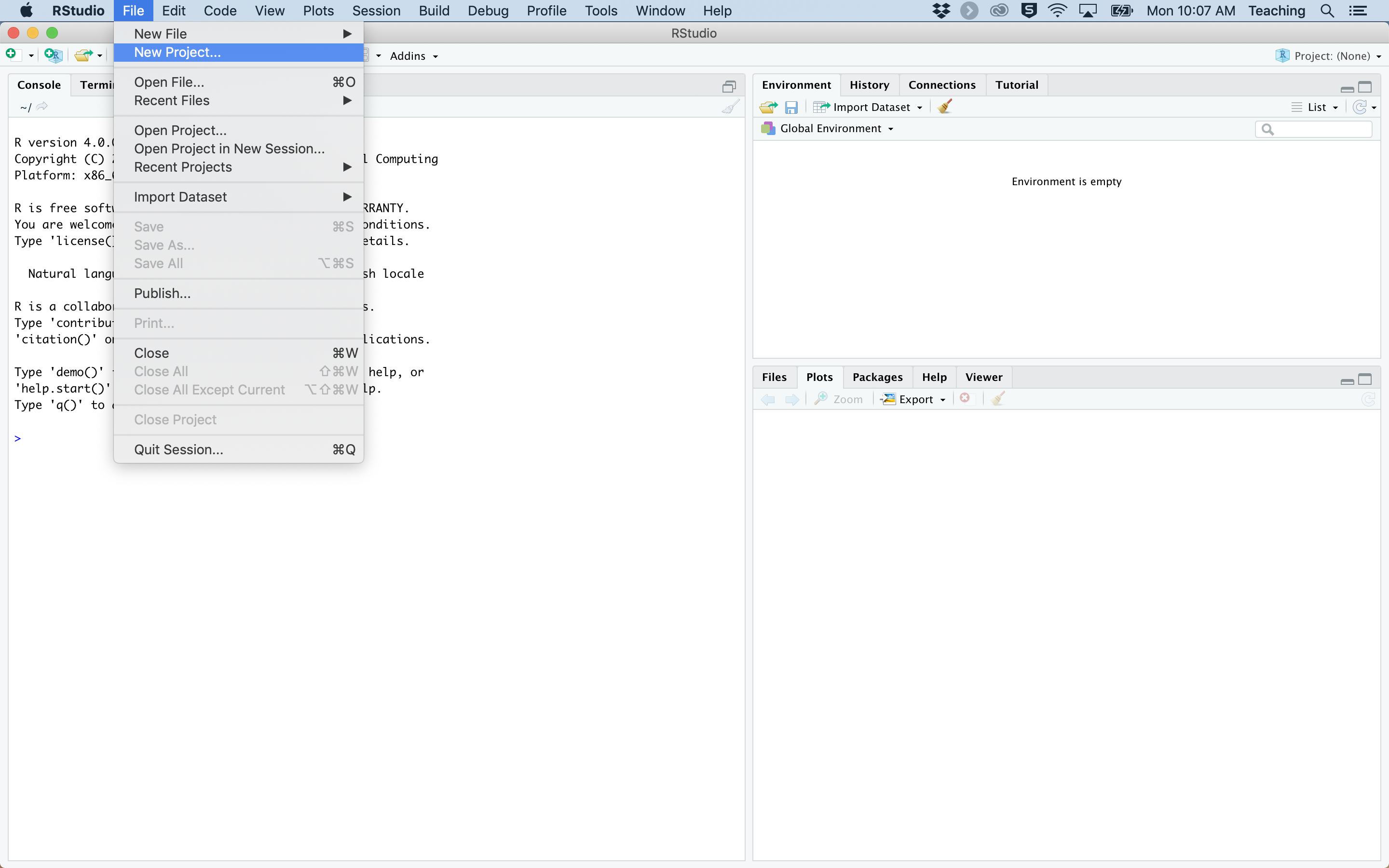
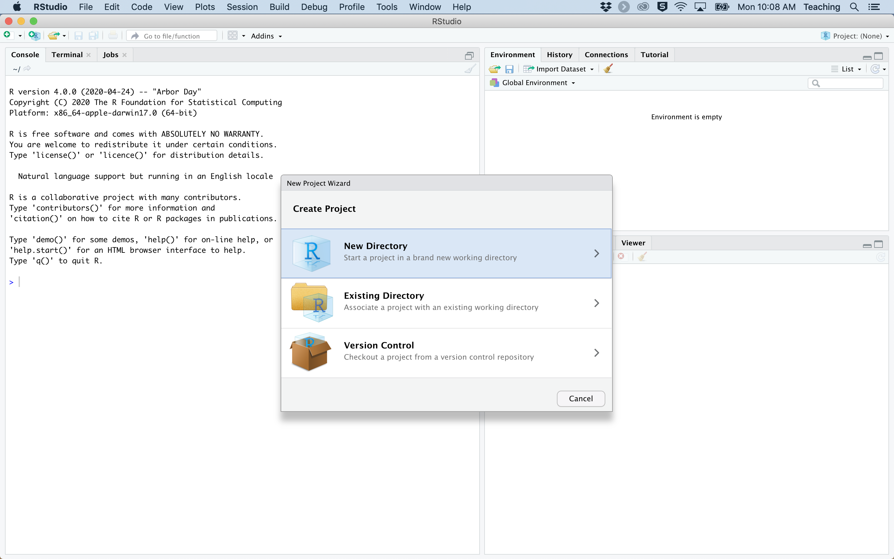
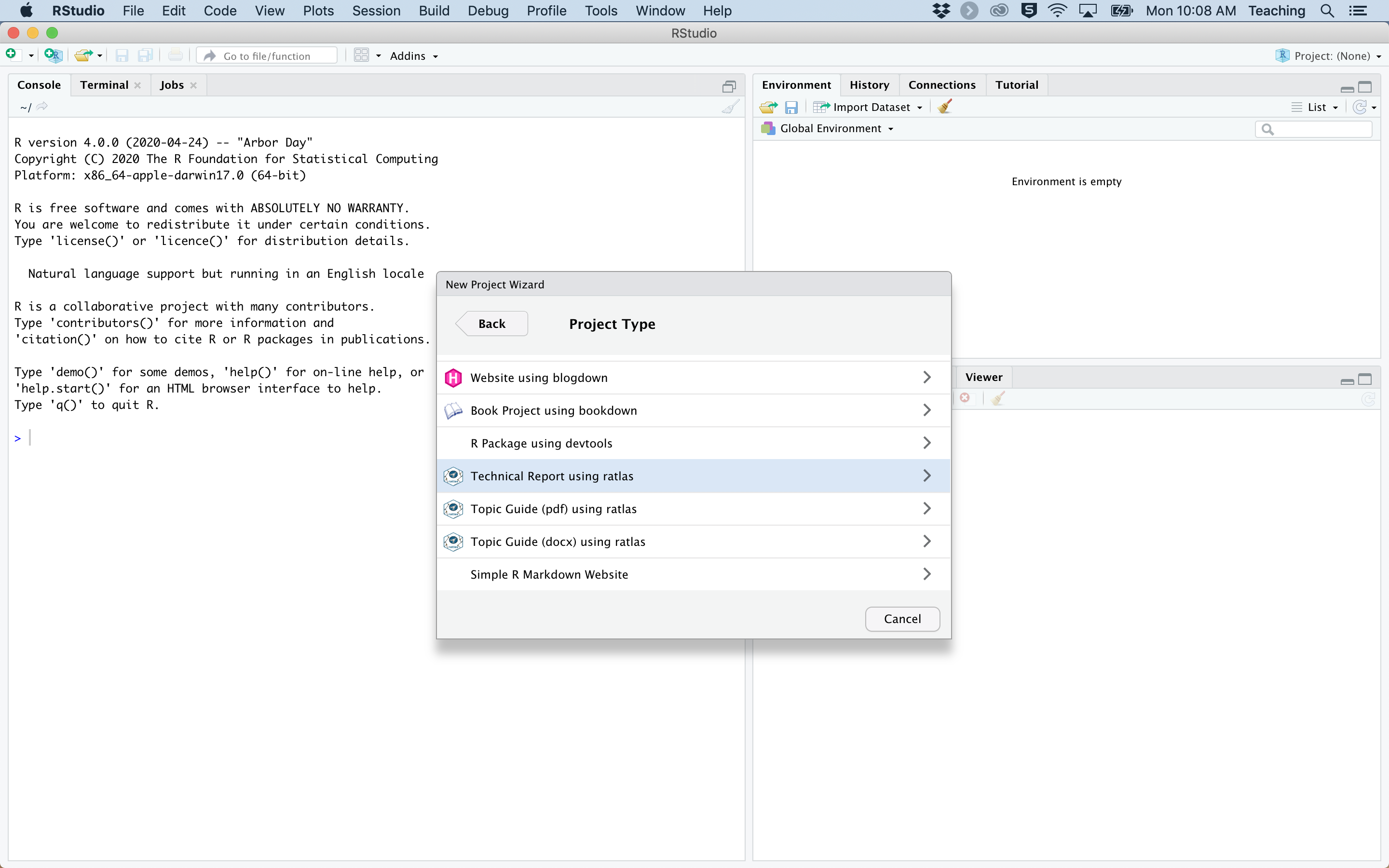
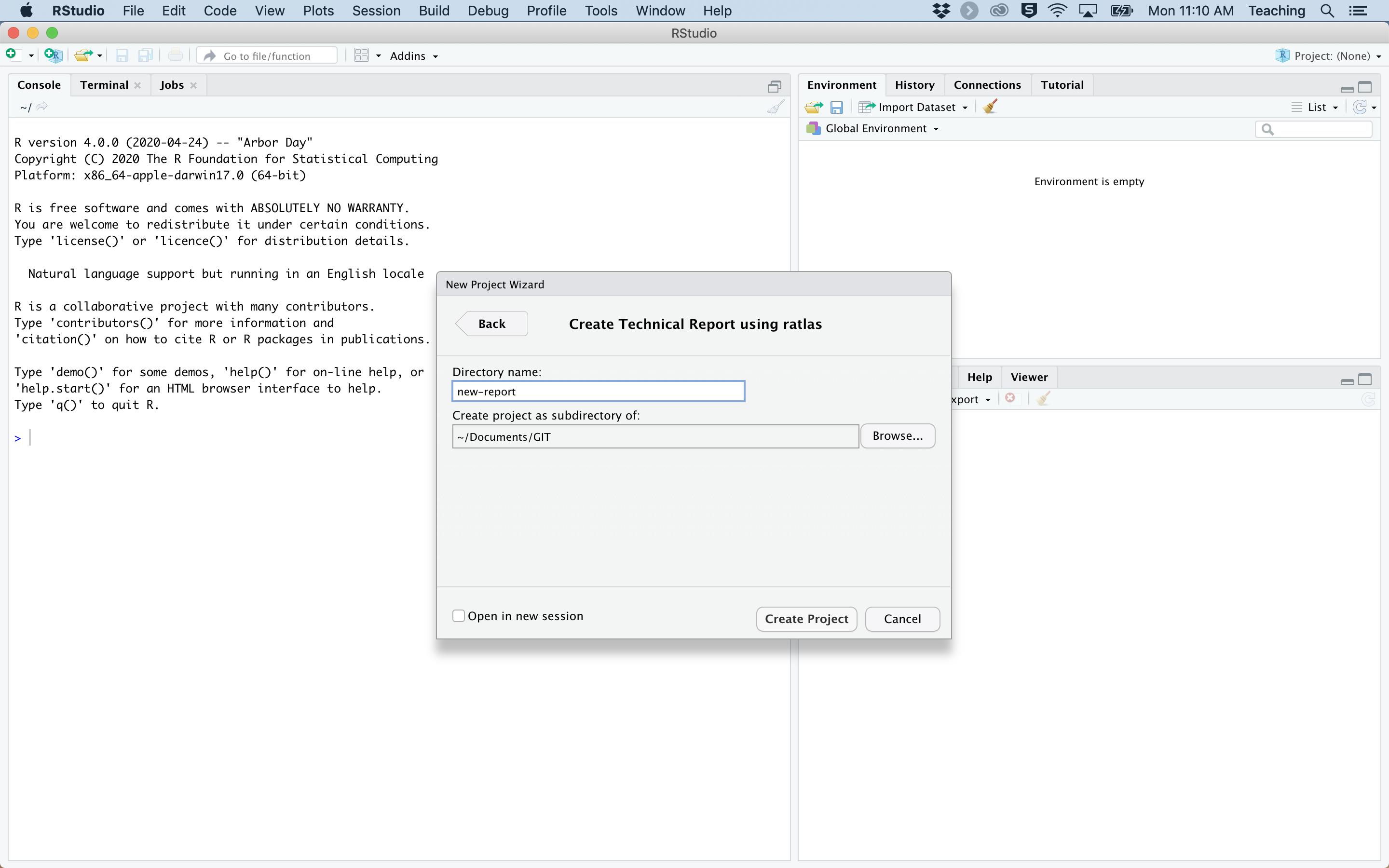
Figure 1: Process for creating a new report with {ratlas}.
Your new project should open automatically. You can then open the R Markdown document by clicking the .Rmd file in the Files pane of the RStudio window. The .Rmd document will automatically be named with the name you gave your project. This will open up a document that looks similar to Figure 2.
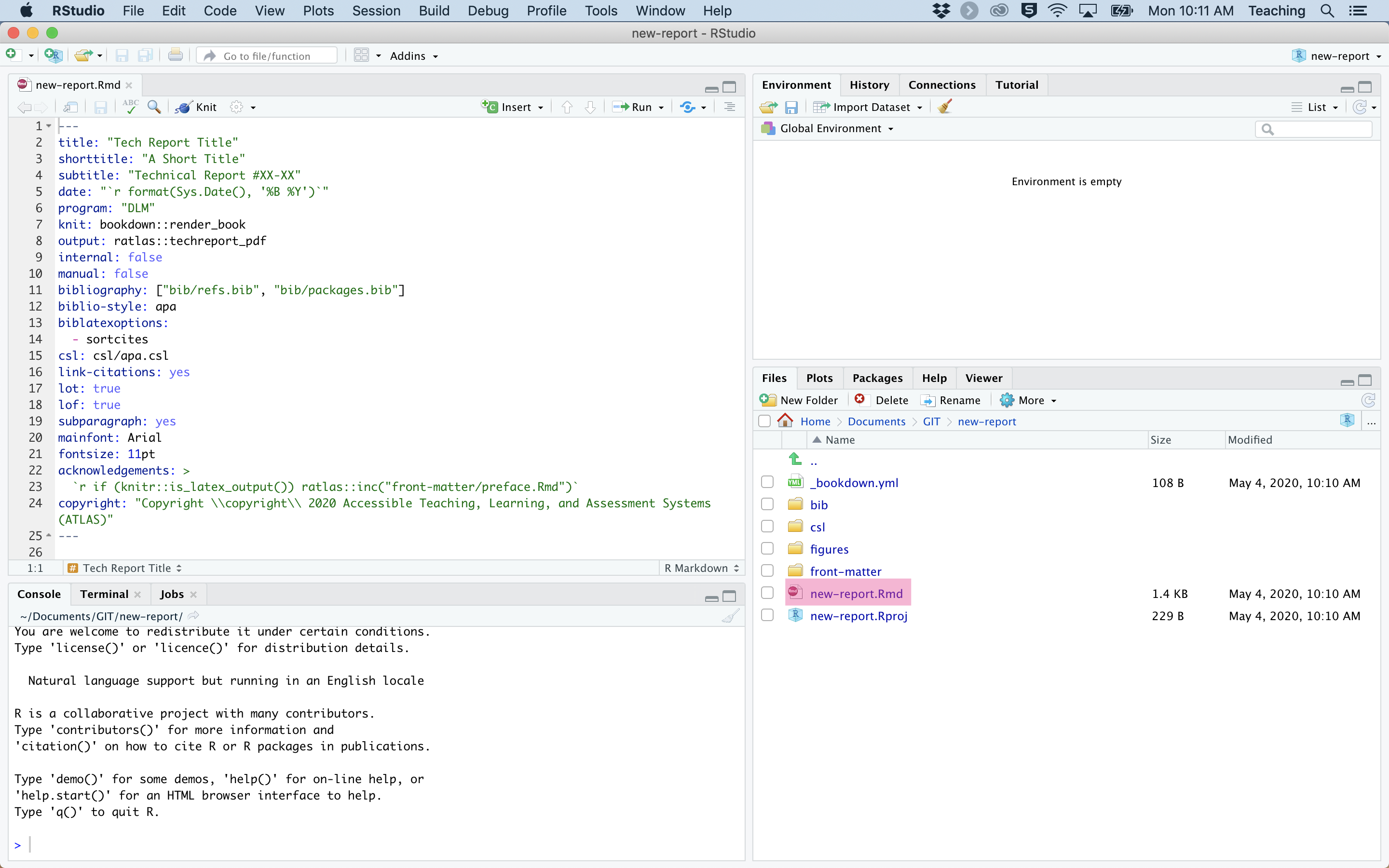
Figure 2: Open the R Markdown file.
At this point, it’s good practice to try generating the template report. We haven’t made any changes, so generating the document using this template file ensures that your system is set up correctly. You can generate the document by pressing the Knit button in RStudio, as shown in Figure 3.
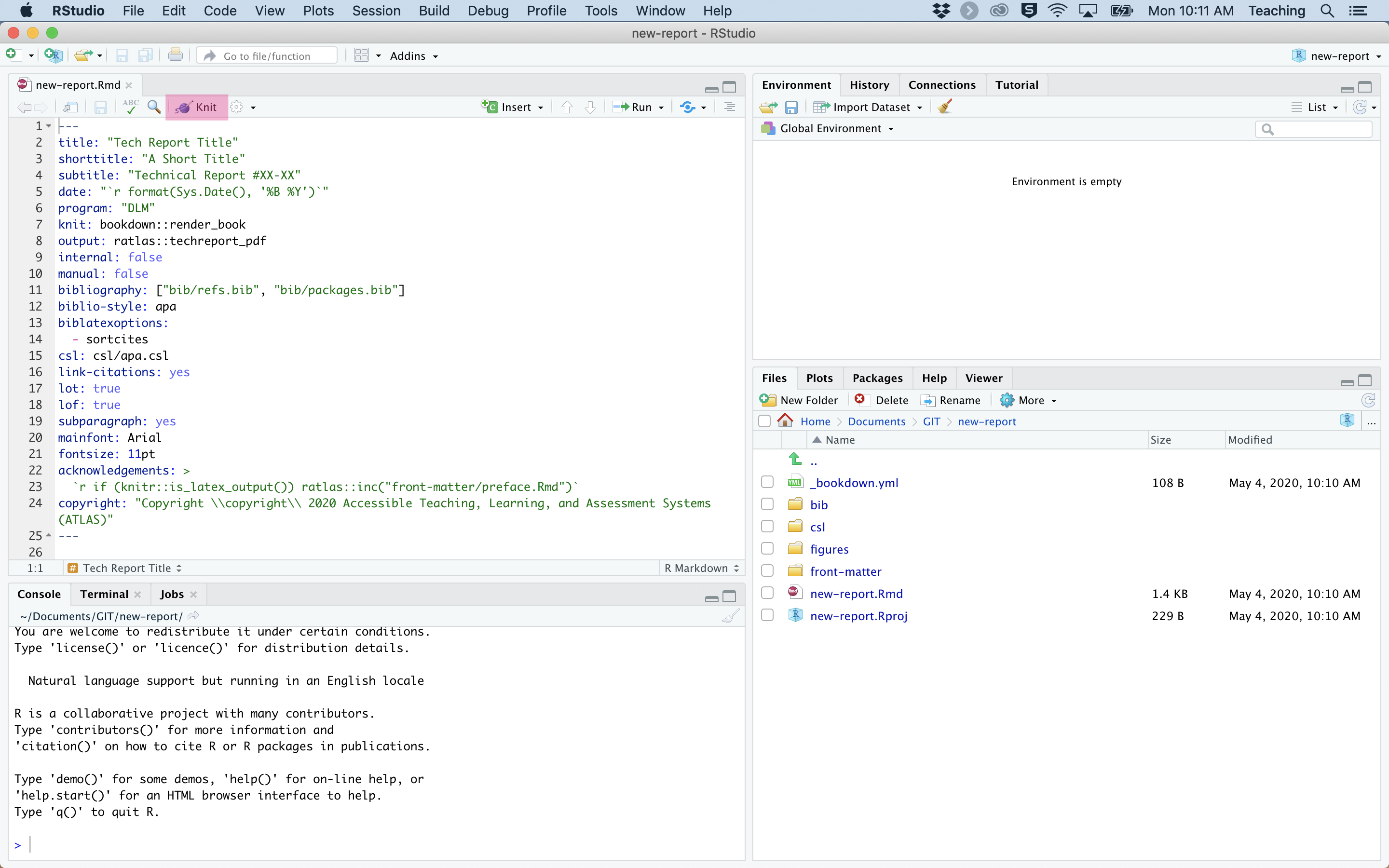
Figure 3: Generate your document using the Knit button.
Editing the Report
Once the document successfully generates, you’re ready to begin editing the template. The first place to start is the meta data at the top of the .Rmd file. This is known as the YAML header, because this information follows YAML (YAML Ain’t Markup Language) syntax. The default YAML header for a technical report is shown in Figure 4.
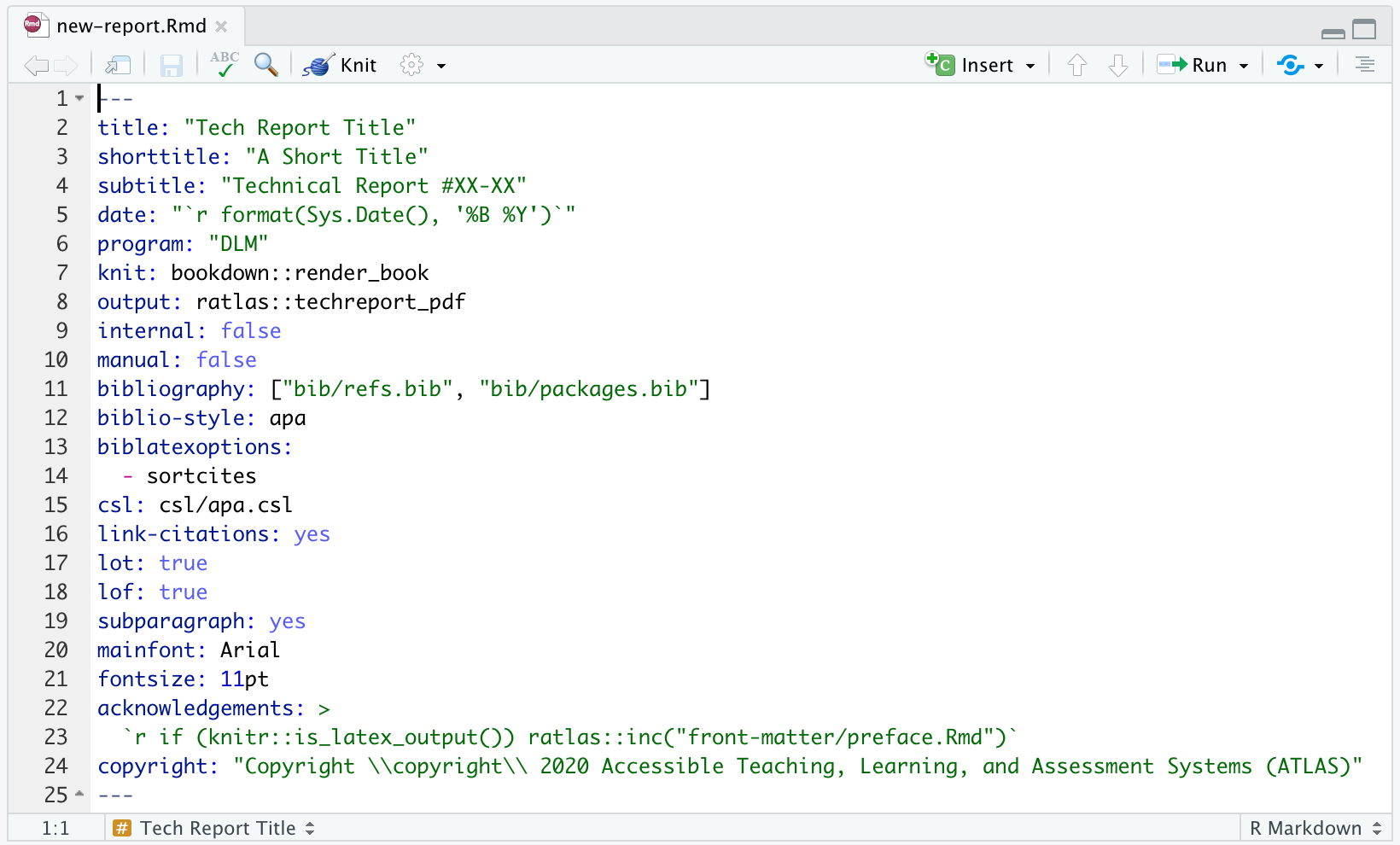
Figure 4: The default YAML header for a technical report.
The following fields should be edited:
-
title: The title of the report. -
shorttitle: An abbreviated title that will appear in the report header. -
subtitle: The report type (i.e., Technical or Research) and number.
Other fields are optional:
-
date: The default is to populate the current month and year. This can be hard coded (e.g.,date: "May 2020") is desired. -
program: The default is"DLM", but {ratlas} also supports"ATLAS"and"I-SMART"reports. The main effect is to change the branding on the cover page. -
internal: Is the report for internal use only? Iftrue, additional language is added to the footer. -
manual: Is this document a technical manual? If true, additional formatting options are applied (e.g., each major section starts on a new page). -
bibliography: A list of.bibfiles containing references for the report. See References for additional information. -
lot: Should a list of tables be included? The default istrue. -
lof: Should a list of figures be included? The default istrue. -
copyright: The copyright statement to include at the bottom of cover page. In most cases this should not need to be edited.
All other fields should not be edited, as they provided additional meta data to control how the output document is generated.
Directly beneath the YAML header is an R code chunk called setup, which is shown in Figure 5.
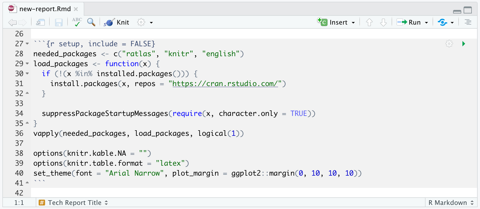
Figure 5: The default setup chunk for a new report.
In most cases, only the first line of the setup chunk will need to be edited. This defines the R packages that are needed for your report. If you are just writing text and not doing any analysis, you can probably leave this as is. However, if you are including your analysis in this document (highly recommended), or plan make tables or figures, you may need to add additional packages here. The rest of the setup chunk loads the specified packages, sets some default options for table output, and sets a default theme for any plots made with ggplot2. If there are other options or settings you need to apply to your whole report, this is the place to them.
Writing in Markdown
Now that all of the setup is complete, it’s time to start writing! R Markdown uses the Markdown language for formatting text. The only difference between writing in Markdown and a more traditional editor (e.g., Microsoft Word) is that in Markdown all of the formatting is included directly in the text. For example, if you want to put a word in italics, you wrap the word in asterisks so that *here are some italics* becomes here are some italics. The most common formatting options are:
- Make headings with
#(e.g.,# Level 1 Heading,## Level 2 Heading, etc.) - Make italics with one asterisk or underscore (e.g.,
*italics*or_italics_) - Make bold with two asterisks or underscores (e.g.,
**bold**or__bold__) - Make in-line code by wrapping text in back ticks (e.g.,
`code`) - Create links using
[text](link)(e.g.,Visit the [DLM website](https://dynamiclearningmaps.org).)
You can also create a bulleted list using asterisks or hyphens.
- item 1
- item 2
    - item 2.1
    - item 2.2
For more in-depth descriptions of Markdown formatting, check out Chapter 2 of bookdown: Authoring Books and Technical Documents with R Markdown and the R Markdown website.
Adding Tables
There are many ways to create professional tables in R Markdown. We recommend using knitr::kable() and the {kableExtra} package. The first step is to your data into data frame. You can either read the data in from a file or create the data manually.
my_data <- tribble(
  ~label,     ~count,  ~percent,  ~correlation, ~pvalue,
  "Group 1",    103L,      0.92,        -0.895,   0.120,
  "Group 2",   1064L,      32.1,         0.051,   0.030,
  "Group 3",  79205L,      95.4,         0.927,   0.001
)
my_data
#> # A tibble: 3 × 5
#>   label   count percent correlation pvalue
#>   <chr>   <int>   <dbl>       <dbl>  <dbl>
#> 1 Group 1   103    0.92      -0.895  0.12
#> 2 Group 2  1064   32.1        0.051  0.03
#> 3 Group 3 79205   95.4        0.927  0.001
The next step is to format the table for printing. The fmt_table() function will apply default formatting and work in most cases. Notice the formatting that has been applied below. Commas have been added to integer values, decimal digits have been rounded to the same number of decimal places, and leading zeros have been removed from values that are bounded between -1 and 1. Leading and trailing spaces have also been added so that values will be centered and decimal aligned in the table. See ?ratlas::formatting for specific formatting options that are wrapped by fmt_table(). These formatting functions can be used to specific styling of columns that do not conform to the defaults specified in fmt_table().
my_data %>%
fmt_table(corr_dig = 2, prop_dig = 2)
#> # A tibble: 3 × 5
#> label count percent correlation pvalue
#> <chr> <chr> <chr> <chr> <chr>
#> 1 Group 1 "\\ \\ \\ \\ \\ 103" "\\ \\ 0.9" "−.90\\ \\ " ".12"
#> 2 Group 2 "\\ \\ 1,064" "32.1" ".05" ".03"
#> 3 Group 3 "79,205" "95.4" ".93" "<.01\\ \\ \\ "The table can then be created using knitr::kable(). There are several arguments supplied to the kable() function. The align argument specifies the alignment of each column. Because we formatted the table with fmt_table(), we can set the alignment of all the numeric columns to "c" (centered). The booktabs and linesep arguments control the appearance of the table. By setting escape = FALSE, we tell the kable() function to not escape special characters, allowing for the padding spaces we added to remain in tact. Additionally, column names for the table and a caption are specified. The last step is to add additional styling from the {kableExtra} package. In this example, we use the kableExtra::kable_styling() function to set some \(\LaTeX\) options. Specifically, the "HOLD_position" setting ensures that the table will appear in the exact position of the code chunk (i.e., the \(\LaTeX\) engine is not allowed to float the table above or below additional paragraphs in order to avoid extraneous white space). For more customization options with the {kableExtra} package, see the package vignettes for HTML and PDF tables.
my_data %>%
  fmt_table(corr_dig = 2, prop_dig = 2) %>%
  kable(align = c("l", rep("c", 4)), booktabs = TRUE, linesep = "",
        escape = FALSE,
        col.names = c("Group", "Students (*n*)", "\\%", "*r*", "*p*-value"),
        caption = "An example table") %>%
kable_styling(latex_options = "HOLD_position")| Group | Students (n) | % | r | p-value |
|---|---|---|---|---|
| Group 1 | 103 | 0.9 | −.90 | .12 |
| Group 2 | 1,064 | 32.1 | .05 | .03 |
| Group 3 | 79,205 | 95.4 | .93 | <.01 |
Finally, we can cross reference the table using the chunk label. For example, the full code chunk to create Table 1 is shown below. Cross references for tables are created using the syntax \@ref(tab:chunk-label). For example, Table \@ref(tab:example-table) renders as Table 1. For more on cross references see this section from bookdown: Authoring Books and Technical Documents with R Markdown and this section from the R Markdown Cookbook.
Adding Figures
Figures can be created using the ggplot2 package in R. For example, we can use the iris data set that is built into R to create a scatter plot, which is shown in Figure 6. For additional details on creating figures with {ratlas}, see vignette("plotting").
ggplot(iris, aes(x = Petal.Length, y = Sepal.Length, color = Species)) +
  geom_point() +
  labs(x = "Petal Length", y = "Sepal Length") +
  scale_color_okabeito() +
  theme_atlas()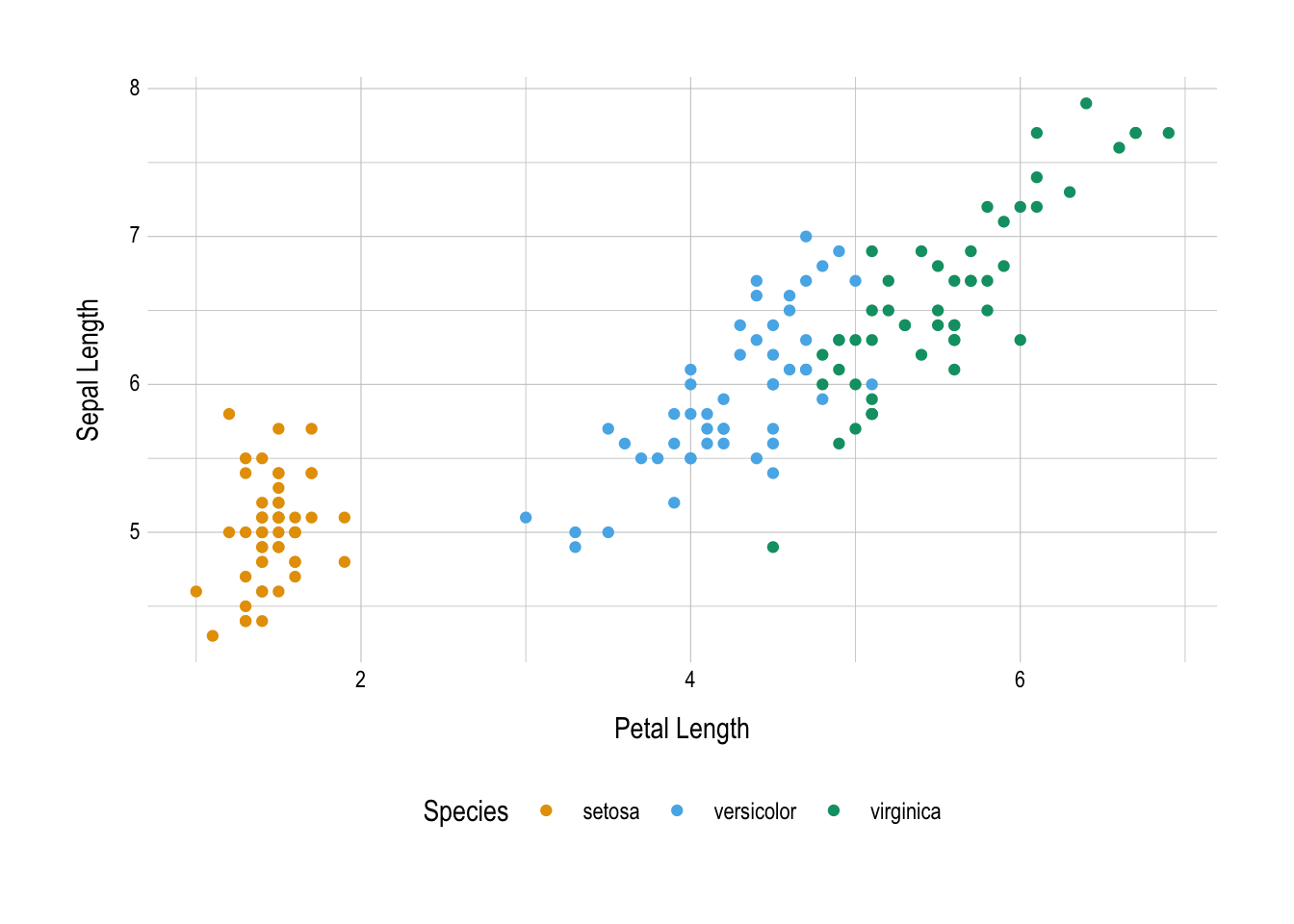
Figure 6: An example figure.
As with tables, we can create cross references for figures. For figures, the caption must be specified as a chunk option, as shown below. Then, we can create a cross reference using the same syntax that was used for tables, replacing tab: with fig:. That is, Figure \@ref(fig:example-figure) will render as Figure 6.
```{r example-figure, fig.cap = "An example figure."}
ggplot(iris, aes(x = Petal.Length, y = Sepal.Length, color = Species)) +
  geom_point() +
  labs(x = "Petal Length", y = "Sepal Length") +
  scale_color_okabeito() +
  theme_atlas()
```
Citations
The last major category of features for report writing is citations. The first step for including citations is to format your references into a .bib file. Reference managers such as EndNote or Zotero offer the option to export references to a .bib file (e.g., Bibtex), making this step easier. Entries in a .bib file should look like the following example. The first line contains important metadata. The @article specifies the type of reference and will control what type of information is included in the printed bibliography. The string directly after the opening brace (i.e., lcdm) is the citation key. This is what we’ll use to actually make a citation. Both of these pieces of metadata will be automatically generated by your reference manager. If you are writing your own .bib file, or need to manually insert an entry, you can find many examples here.
@article{lcdm,
  author = {Henson, Robert A. and Templin, Jonathan L. and Willse, John T.},
  year = {2009},
  title = {Defining a family of cognitive diagnosis models using log-linear models with latent variables},
  journal = {Psychometrika},
  volume = {74},
  pages = {191--210},
  doi = {10.1007/S11336-008-9089-5}
}
The next step is to tell R Markdown about your .bib files. The YAML header includes a bibliography field, where we specify the .bib files. In the template file, we assume that .bib files are kept in a bib/ directory. Your references are saved in bib/refs.bib. By default, the template will write out a separate .bib file, bib/packages.bib that includes the citation information for all the R packages you have loaded, making it easy to cite your software. You can add more .bib files if that makes organizing easier. The YAML header also includes extra metadata about how references should be formatted. The default is to use APA style. You can find .csl files for other citation files here if APA is not suitable.
---
...
bibliography: ["bib/refs.bib", "bib/packages.bib"]
biblio-style: apa
csl: csl/apa.csl
...
---
We are then ready to start making citations. Citations are made using the syntax @citation-key. For R packages, the citation key is always R-pkgname (e.g., R-ratlas). To make a parenthetical citation, place the citation key within brackets (e.g., [@R-ratlas]). In-text citations can be made by remove the brackets. The author can be suppressed by adding a minus sign before the key (e.g., -@R-ratlas). Multiple citations are separate by semicolons. Finally, additional text can be added before or after a citation by using a semicolon or commas as appropriate. Table 2 shows some common citation styles, along with the code to generate the style.
| Code | Renders as… |
|---|---|
[@R-ratlas]
|
(Thompson et al., 2025) |
@R-ratlas
|
Thompson et al. (2025) |
[LCDM; @lcdm]
|
[LCDM; Henson et al. (2009)] |
[-@lcdm]
|
(2009) |
[@lcdm, pp. 3]
|
(Henson et al., 2009, p. 3) |
@lcdm [p. 3]
|
Henson et al. (2009, p. 3) |
[@lcdm; @R-ratlas]
|
(Henson et al., 2009; Thompson et al., 2025) |
Full references for all citations that have mentioned in the text are automatically added to the end of the document. This means that you only need to worry about making your citations within the text. The bibliography is handled automatically by R Markdown. For more information on citations, see the R Markdown website and the R Markdown Cookbook.
Best Practices
In the final section, we include some recommendations and best practices for writing reports in R Markdown that will make life for you and your collaborators easier.
File paths
Nothing is worse than getting some code from a collaborator, attempting to run it, and seeing an error that says the data file does not exist. This is most likely due to file path issues. For example, the file /Users/myname/Documents/my-project/some-data.csv will not exist on your computer, because you have a different name. If you use a different operating system, the beginning of the file path may be completely different (i.e., C:\ vs. /). This is problematic for two reasons:
- I have to go through and replace all the file paths before I can run your code.
- When I send the code back, you have to change all the files paths back.
Luckily, the {here} package is here (no pun intended) to save the day. When you create a new report using the process described above, an R project is automatically created (you should see a .Rproj file in your directory). The {here} package works by building file paths relative to the directory where the .Rproj file is. Let’s look at an example. Say I have the following file structure for my project:
/Users/jake/GIT/projects/simulation-study/
├── data
│   ├── some-data.csv
│   ├── random-seeds.rds
├── my-proj.Rproj
├── my-report.Rmd
├── output
│   └── all-output.rds
├── R
│   └── simulation.R
In this project, there is a data/ directory with raw data, an R/ directory where the analysis code lives, and an output/ directory, where the results from the analysis are saved. The report lives in the my-report.Rmd file. When writing the report, I will likely need to read in the results. One option is to use read_rds("/Users/jake/GIT/projects/simulation-study/output/all-output.rds"). However, we know that this will break on other machines. Instead, we can use read_rds(here("output", "all-output.rds")). This will look for the .Rproj file, and from there, look for an output directory with an all-output.rds file. This way, when another collaborator downloads the project, the file paths will “just work.” For more information on file paths and why the {here} package is important, see this blog post from Jenny Bryan.
In-Line Output
If at all possible, you should avoid the hard coding of numbers. For example, let’s say we have some data on cars and estimate the following model:
my_data
#> # A tibble: 32 × 3
#>      mpg  disp   cyl
#>    <dbl> <dbl> <dbl>
#>  1  21    160      6
#>  2  21    160      6
#>  3  22.8  108      4
#>  4  21.4  258      6
#>  5  18.7  360      8
#>  6  18.1  225      6
#>  7  14.3  360      8
#>  8  24.4  147.     4
#>  9  22.8  141.     4
#> 10  19.2  168.     6
#> # ℹ 22 more rows

lm_mod <- lm(mpg ~ disp + cyl, data = my_data)
coef(lm_mod)
#> (Intercept)        disp         cyl
#> 34.66099474 -0.02058363 -1.58727681
When reporting the coefficient for cyl we might say, “Keeping displacement constant, an additional cylinder is associated with a loss of about 1.6 miles-per-gallon.” But now let’s say that the data file gets updated:
my_new_data
#> # A tibble: 48 × 3
#>      mpg  disp   cyl
#>    <dbl> <dbl> <dbl>
#>  1  17.3  276.     8
#>  2  15.2  304      8
#>  3  16.4  276.     8
#>  4  15    301      8
#>  5  18.7  360      8
#>  6  18.1  225      6
#>  7  10.4  472      8
#>  8  10.4  472      8
#>  9  15    301      8
#> 10  21.4  258      6
#> # ℹ 38 more rows
Notice that we now have 48 rows instead of 32. If we re-estimate the model, we can see the coefficients have changed:
lm_mod <- lm(mpg ~ disp + cyl, data = my_new_data)
coef(lm_mod)
#> (Intercept)        disp         cyl
#> 26.90384800 -0.01829298 -0.66756073
We now have to go through all of our text to replace any numbers that depend on the data set (e.g. sample size) or analyses (e.g., coefficients). This can be a tedious process, and result in errors if any numbers are missed. Instead, we should use in-line R expressions to automatically populate these numbers. For example, we can populate the cyl coefficient using `r fmt_digits(coef(lm_mod)["cyl"], 1)`, which will render as -0.7. This way, no matter how much the data changes, or if the model is altered, the text of the report will always populate with the most correct, most up-to-date value.
Additional Helpers
There are two additional helpers that may be useful for automatically populating the text of a report. First, knitr::combine_words() can be used to create a comma separated character string from a vector of values. For example, `r combine_words(c("one", "two", "three"))` becomes one, two, and three.
Finally, APA style specifies that integer values less than ten should be spelled out (i.e., “two” instead of 2). The {english} package can be used to translate numbers to words. For example `r words(3)` becomes three. For more details on the {english} package, see vignette("the-english-patient", package = "english").
Keep Learning
There are many resources available for learning more about writing reports with R Markdown. Here are a few free resources that I have found particularly helpful:
- For a high-level overview of everything you could ever want to know about R Markdown, see R Markdown: The Definitive Guide, by Yihui Xie, J. J. Allaire, and Garrett Grolemund.
- For more details and help with {bookdown}, the R Markdown extension used by {ratlas}, see bookdown: Authoring books and technical documents with R Markdown, by Yihui Xie.
- For quick recipes for formatting and customizing R Markdown documents, see the R Markdown Cookbook, by Yihui Xie and Christophe Dervieux.
There are also many resources for getting started with data analysis and programming in R:
- For a friendly introduction to R, see Hands-On Programming With R, by Garrett Grolemund.
- For a general introduction to doing data science in R, see R for Data Science (including a section specifically on communicating with R Markdown), by Hadley Wickham and Garrett Grolemund.
- For quick recipes to accomplish various tasks in R, see the R Cookbook, by JD Long and Paul Teetor
- For an introduction to statistical inference in R, see Statistical Inference via Data Science: A ModernDive into R and the tidyverse, by Chester Ismay and Albert Y. Kim.